Precipitation Spatial Average

Problem

Precipitation estimates over large areas are needed for many purposes, yet precipitation is typically only measured at points in small buckets. How do we estimate the spatial average precipitation for a large area using point measurements?

Goal

The goal of this exercise is to calculate the total annual depth of precipitation in the DCEW by averaging weighing bucket gauge data from meteorological stations using the hypsometric method, Thiessen polygons, and direct averaging.

Learning objectives

Upon completion of this exercise, students will be able to:

• Describe the weighted average approach for estimating the average precipitation over a watershed from multiple gauges
• Obtain weight factors using hypsometric, Thiessen polygon, and direct average methods
• Construct Thiessen polygons
• Construct a hypsometric function from a histogram of elevation data
• Develop a mathematical equation expressing the relationship between precipitation and elevation
• Combine a hypsometric function with a precipitation-elevation relationship to produce an elevation weighted average precipitation depth

Project Files

• EXCEL workbook 

Requirements and Connections

• This exercise requires historical hourly precipitation data collected from meteorological stations at varied elevations within DCEW.
• Products of this exercise may be used by the Watershed Water Balance exercise.

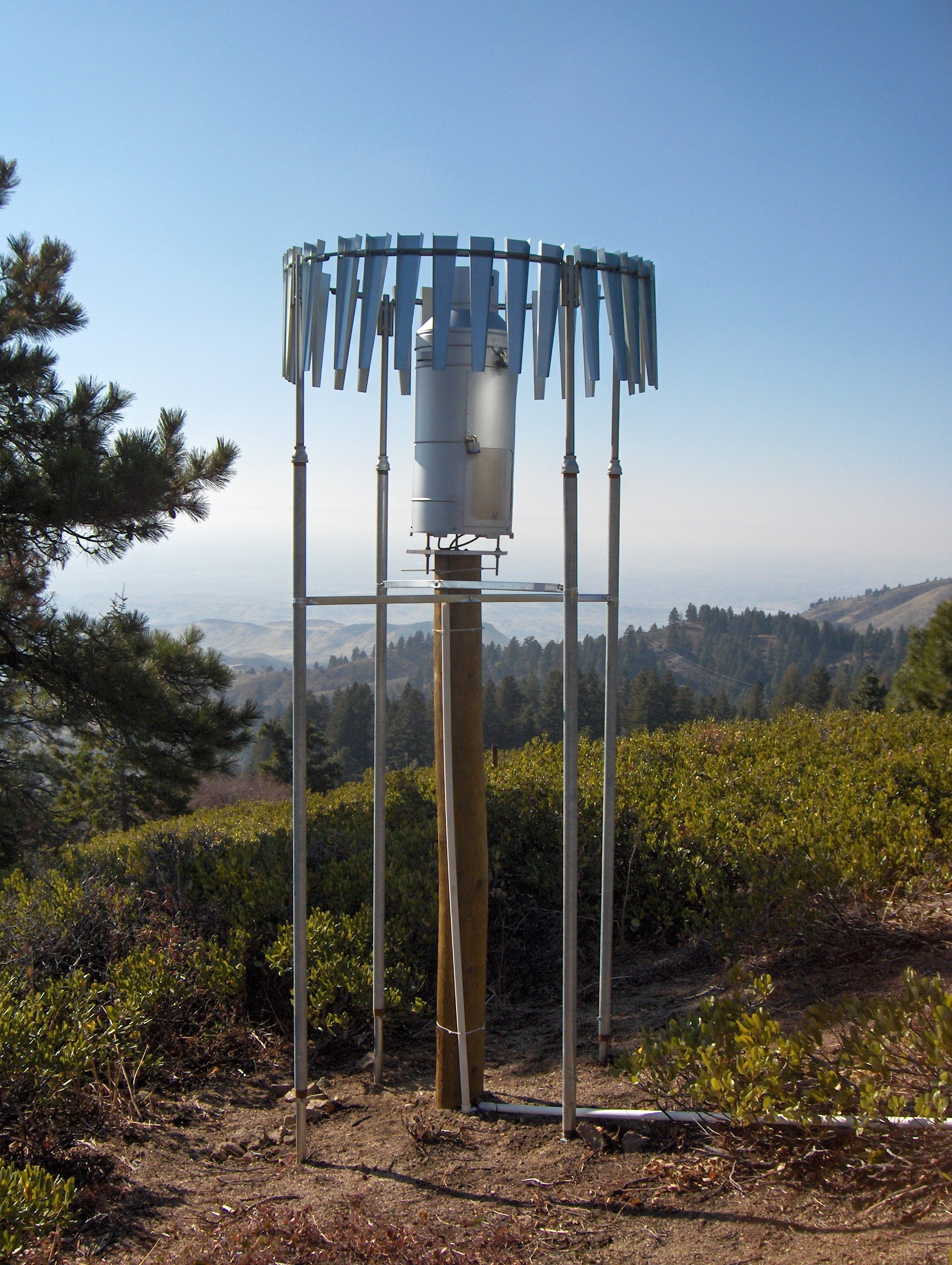
Precipitation is typically measured in tipping or weighing bucket gauges 8-12 inches diameter. Hydrologists, however, are interested in precipitation over a region or watershed. If there were no spatial variability in precipitation, a single bucket in a watershed would be sufficient. This is not the case. Precipitation is highly variable. When multiple gauges area available, the spatial average precipitation must be calculated from point measurements.  A weighed average approach is commonly used:

where P is the precipitation measured at a gauge (g), G is the total number of gauges, and w is the weight assigned to a gauge. Most common approaches to estimate spatial average of multiple gauges are simply methods to assign weights. For example, we could elect to simply take the direct average of all of our gauges. In this case, each gauge gets an equal weight. If G = 3, each gauge gets a weight of 1/3. This is the same as same as simply adding up each P and dividing by the number of gauges.

A problem with the direct averaging approach is it assumes that the gauges are placed in a way that captures the actual spatial variability. For example, we know that in mountainous terrain precipitation tends to be higher at higher elevations in a watershed. If all of our gauges are placed at high elevations, we will overestimate the average. If the gauges, however, are placed throughout the watershed in a way that appropriately represents the relationship between precipitation and elevation, our direct average will be more accurate. This, however, is not commonly possible. Instead, we can use the hypsometric method. The term hypsometry refers to the measurement of elevation.

The hypsometric method combines the distribution of elevation within a watershed with a know relationship between precipitation and elevation to determine weights for elevation classes. Other commonly used methods to assign weights include Thiessen polygons based on proximity of gauges,   and isohyetal methods based on precipitation contours. An advantage of the hypsometric method in mountainous terrain is that is accounts for the mechanism that is known to produce spatial variability of precipitation.

Hypsometric Method: Developing the Precipitation-Elevation function

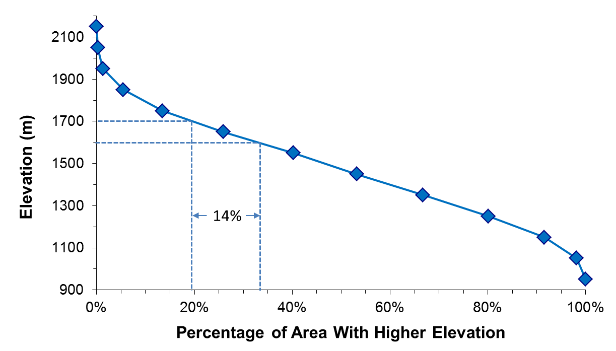
The hypsometric method for estimating spatial average precipitation uses a known relationship between precipitation and elevation (Figure 1) with a known distribution of elevations within a watershed (Figure 2).  Figure 1 tells us how much precipitation falls at an elevation, or within an elevation zone, and Figure 2 tells us how much of a watershed area is within an elevation zone. In other words, the equation in Figure 1 replaces the gauges and Figure 2 provides the weights.

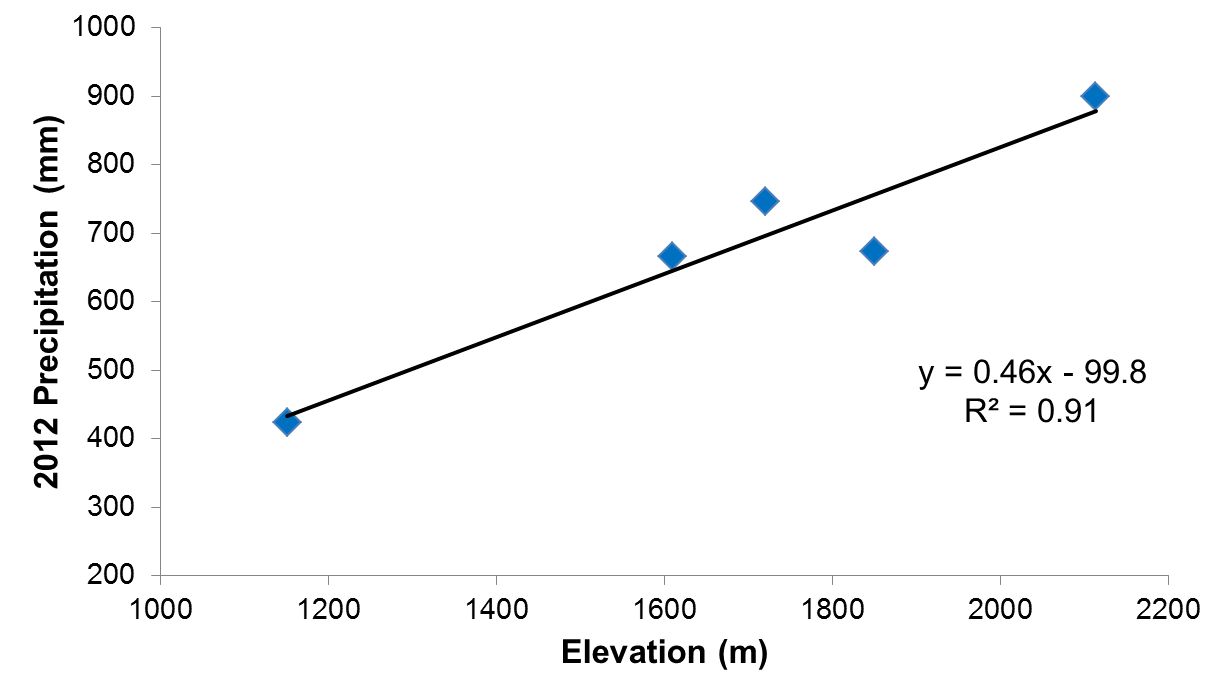
The precipitation-elevation function is often called the orographic equation after the orographic effect that causes precipitation to increase with elevation. If precipitation gauges are distribution along an elevation range with a watershed, we can obtain a mathematical relationship between the elevation of the gauge and the total precipitation collected by the gauge for a specified time period. Most commonly, the specified time period is one year. It is important to recognize the precipitation-elevation equations can only be applied at time periods for which they were developed. If total annual precipitation was used to develop the equation, the equation cannot be applied to specific storms, seasons, or any other sub-annual time period. Nor should equations from one year be applied to another year, or from one watershed to another watershed. These latter statements are guidelines rather than rules. Although not ideal, it may not be a bad assumption that the precipitation-elevation remains relatively stable from year to year, or that neighboring watershed may be represented by similar functions.
Most certainly, however, a precipitation-elevation function from the foothills near Boise Idaho should not be used to model precipitation in Idaho’s Sawtooth Mountains.

After gathering precipitation totals for each gauge, the mathematical equation can be developed. Most commonly, a linear equation of the form below is used:

where P is the precipitation measured at gauge g, z is the elevation of gauge g, and a and b are curve fitting parameters. The paramater ‘a‘ can be considered a precipitation gradient (dP/dz). Once the precipitation-elevation is derived, it replaces the gauges in weighting equation described above. We can calculate the precipitation for any elevation within a watershed, essentially giving us an infinite number of gauges. It is then necessary to determine the distribution of z, called the hypsometric function.

Hypsometric Method: Deriving the Hypsometric Function

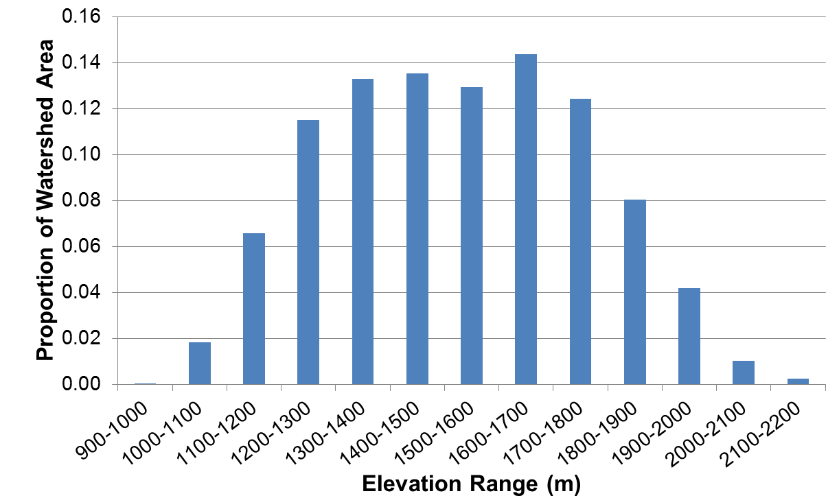
Figure 2 presents a hypsometric function for the DCEW. The y-axis spans the range of elevations found in the DCEW. The x-axis gives the proportion of the watershed area that is above any given elevation. The minimum elevation in the watershed plots at 100%, and the maximum elevation plots at 0%.  The shape of the curve defines the arrangement of elevations between the minimum and maximum.

Use of the hypsometric function to obtain precipitation gauge weights is typically done by discretizing the continuous function into a histogram of elevation zones (Figure 3). For example, Figure 2 shows that 20% of the watershed is higher than 1700 m elevation and 34% of the watershed is higher than 1600 m elevation.  The 1600 m to 1700 m elevation zone therefore occupies 14% of the watershed, as depicted on Figure 3.

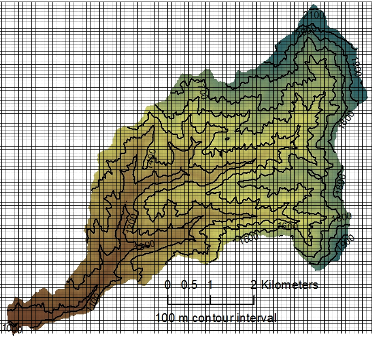
Figures 2 and 3 can be derived by analyzing a Digital Elevation Model as described in the Watershed Delineation exercise, or manually by overlaying a regularly spaced grid on an elevation contour map of the watershed (Figure 4).

The number of grid points within an elevation zone divided by the total number of grid points in the watershed is an estimate of the proportion of the watershed in that elevation zone.

Theisson Polygon Method

In the Thiessen polygon approach, gauges are weighted according their proximity to other gauges. Polygons are drawn around each gauge so that all points within a polygon are closer to the one gauge within the polygon than to any other gauge. Once constructed, the proportion of a polygon relative to the watershed area is used as the gauge weight.

Figures 5 illustrates the steps of the Thiessen Polygon method applied to the Reynolds Creek Experimental Watershed as described in the following steps:

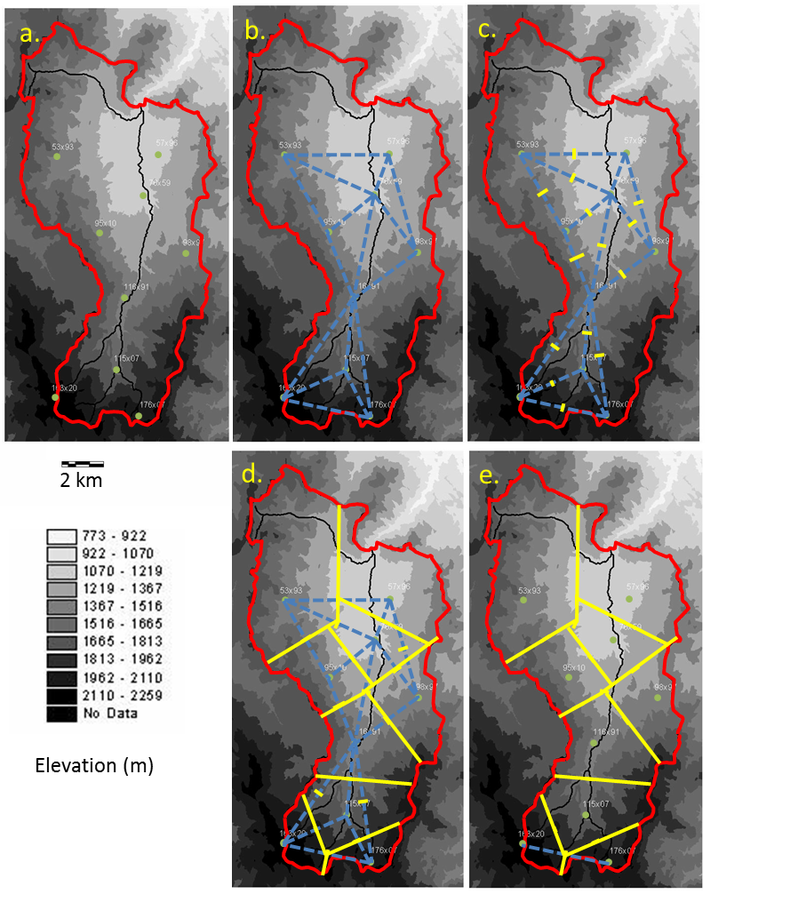
1. On a map with the locations of all gauges (Figure 5a), draw lines connecting adjacent gauges (Figure 5b). Draw lightly with a pencil so that your lines can be erased later. Note that is acceptable to use gauges outside of the watershed boundary.
2. Draw a perpendicular bisector line at the midpoint of each line from step 1 (Figure 5c).
3. From each bisector, draw lines perpendicular to the lines from step 1 until these new lines intersect to form irregular polygons (Figure 5d). This step will take some iteration.
4. When polygons look appropriate, eliminate the connecting lines for clarity (Figure 5e).
5. Measure the relative area of each subregion. Areas can be obtained using a grid-counting approach as described above.

Goal

The goal of this project is to calculate the spatial average depth of DCEW annual precipitation using three weighted average approaches including direct average, hypsometric, and Thiessen methods. You will conduct the analysis on water years 2012, 2013, and 2017.

The instructions below outline specific steps to follow to complete the calculations. Ensure that you understand the problems and goals of this exercise by reviewing the information in the INTRODUCTION and BACKGROUND tabs.

1. Download and prepare data

a. Download this excel workbook which contains precipitation data for the 2012 water year (Oct 1, 2011-Sep 30, 2012) for 3 stations in and adjacent to the DCEW including low elevation (Lower Weather) , mid elevation (Treeline), and high elevation (Bogus Basin) sites. Note that Lower Weather and Treeline meteorological stations are  operated by Boise State, and Bogus Basin is operated by the NRCS SNOTEL network.

b. Review the DCEW site map to see the station locations. Visit the specific site pages above and find the elevation of each station. Enter values (m) in cell B2 of appropriate tabs in the excel workbook.

c. To complete the exercise for WY 2012 skip to Step 2. Otherwise, follow the procedure below to prepare data for additional water years:

• Lower Weather and Treeline stations: Cumulative precipitation data from 2000-2017 for Lower Weather and Treeline sites can be found on the Google Sheet. Note that the cumulative sum resets at January 1st each year. To create water year datasets for each site you will need to determine the cumulative precipitation that occurred from Oct 1 to Dec 31 and then add that amount to the cumulative precipitation that occurred from Jan 1 through Sep 30 the following year. When your water year time series are complete, copy date and precipitation data from the  to the appropriate tabs and columns in the workbook.
• Bogus Basin station: Visit the station website. In the “Select Format” menu select csv. In the  “View Historic” menu select “2012” then select “Water Year”, then Click the “View Historic” button. Repeat for years 2013 and 2017. Open the csv file in excel and view the contents. Cumulative precipitation is in the column labeled Prec.-1 (in). Convert precipitation data to mm and copy into appropriate tabs in the workbook. Note that this station provides daily data while DCEW sites provide hourly data.

2. Compute the spatial average precipitation by direct averaging

A. Investigate each precipitation data set to determine the total depth of precipitation for the year. Enter your values in the appropriate rows in Table 4 in the “Tables” tab.

B. Compute the adirect verage of all stations in Column E of Table 4.

3. Compute the spatial average precipitation by the hypsometric method

A. Develop the precipitation-elevation relationship by following the steps below:

• Open the “Tables” tab in the EXCEL workbook. Enter total annual precipitation for each site in Table 1.
• View the automatically generated scatter chart of Precipitation (y axis) versus Elevation (x axis).
• Determine the linear relationship between Precipitation and Elevation by adding a linear trendline to the chart. Display the regression coefficient and the equation. Enter the equation parameter values in Table 2.
• Repeat for other years as directed by the instructor.

B. Develop the hypsometric function

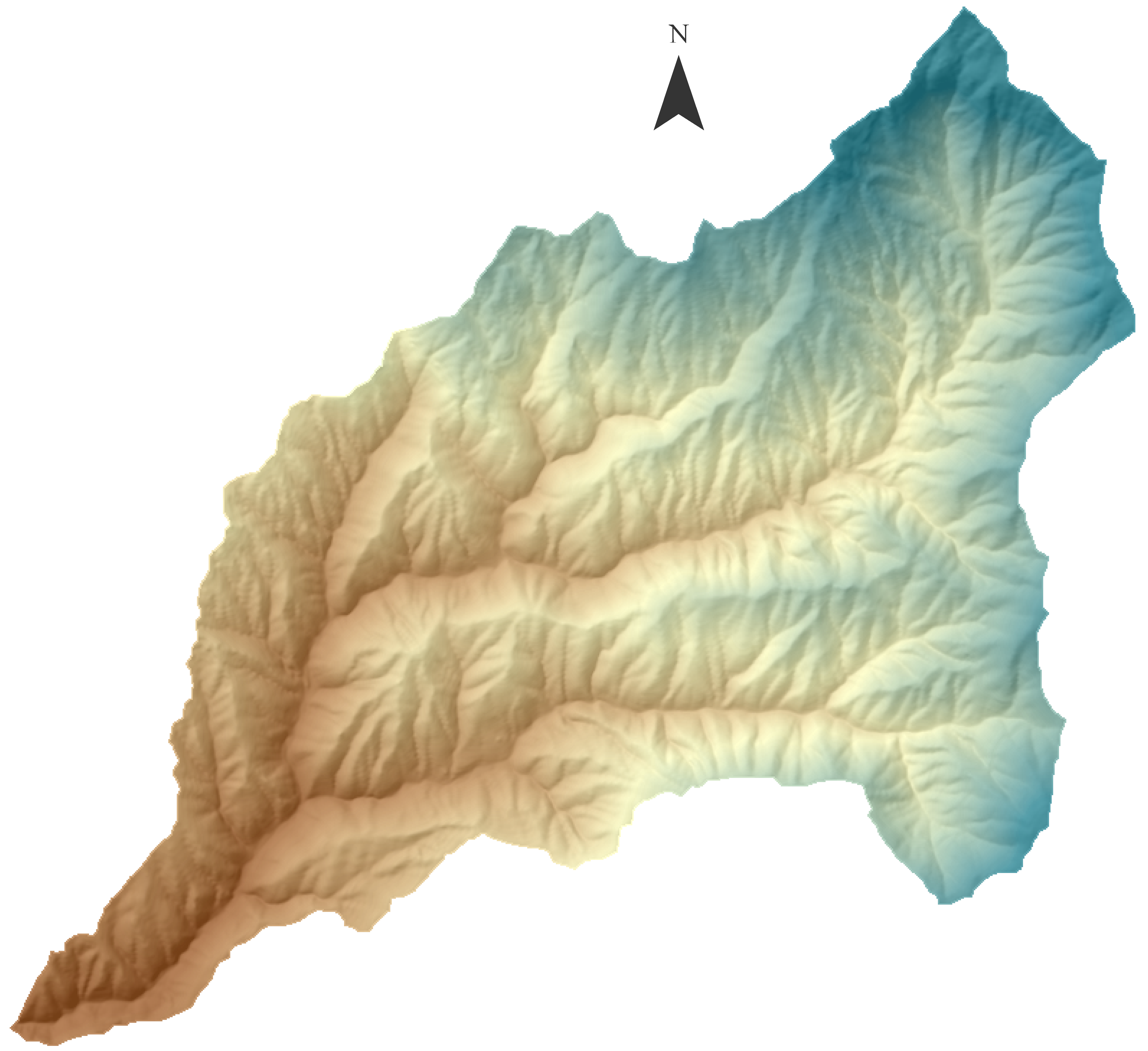
In the “Tables” tab, the ‘Elevation Range’ column in Table 3 contains a list of elevation zones corresponding to those represented in the “Contour Map” tab. Determine the proportion of the watershed in each elevation zone. You can do this manually using a map and grid paper, GIS tools, or a creative way of your choosing:

Grid paper method:

• Overlay the grid provided on the map (in the “Contour Map” tab), and then count the number of cells or points within each zone [see BACKGROUND]; you can count the number of cells/points directly in Excel or by printing the grid-overlaid-image and counting on paper.
• In the ‘Count’ column enter the number of points or cells that exist within each elevation zone.
• In the ‘Weight (Wg)’ column, use the ‘Count’ data to calculate the proportion of the watershed area that is occupied by each elevation zone/

GIS method:

If you are familiar with geographic information systems such as ArcMap or GRASS you can use a  digital elevation model (DEM) to obtain a histogram of elevations classified by elevation zones. Spatial data for Dry Creek are found here: https://earth.boisestate.edu/drycreek/data/spatial-data

C. Calculate the elevation-weighted precipitation

• Construct a hypsometric plot of the catchment similar to Figure 2 in Background. This is not necessary to perform the calculations below, but helps visualize the meaning of the data. According to your plot, what proportion of the catchment are is lower than the Lower Gauge, Treeline, and Bogus stations?
• In the ‘P(z)’ column, use the linear equation parameter values (Table 2) with the ‘Z’ values to calculate the precipitation in each elevation zone. It is important the recognize that in this method, the calculated P(z) values replace gauge values in the Equation 1, the precipitation averaging equation described in [see BACKGROUND]. We now have virtual gauges within each elevation zone.
• Calculate the ‘Wg•P(z)’ within each elevation zone.
• Sum the ‘Wg•P(z)’ values to obtain the  elevation-weighted average precipitation.
• Repeat steps for subsequent years
• Record your answers for all analyzed years in ‘Table 4: Summary Table’ in the “Tables” tab of the workbook provided.

4. Compute the spatial average precipitation using the Thiessen Polygon Method

A. Open the “Theissen Polygon Workshheet” tab in the Excel workbook for this exercise. You will see the map of Dry Creek including all of the monitoring locations. The orange dots indicate the locations of precipitation gauges. You will construct polygons around each of these orange dots. Note that Bogus Ridge is outside of the watershed boundary. Also note that Bogus Ridge is NOT the same as the Bogus Basin site that you used in the Hypsometric method.

B. Follow instructions in the Background section to construct polygons surrounding the following meteorological stations: LW, TL, LDP, SCR, and BR. You can either print the map and construct your polygons with a pencil, or you can export the image to a drawing program and construct the polygons with on a computer. If you use a grid-counting approach to determine polygon areas, record your counts and weights for each polygon in the table provided in the “Thiessen Polygon Worksheet” tab.

C. For each precipitation gauge in step 3b, obtain the total precipitation the 2012 water year.  Record your values in the table provided in the “Thiessen Polygon Worksheet” tab.

D. Using your polygon weights and annual total precipitation values for each gauge, compute the contribution of each polygon to the total precipitation. Sum the precipitation for each polygon to obtain the spatial average precipitation.

4. Discussion Questions

The questions below are prompts to think about issues related to hypsometric method, precipitation measurement, and precipitation variability. Consult your instructor to determine if these or other questions are required.

A. Compare the spatial average precipitation results obtained by the hypsometric, direct average, and if required, thiessen polygon methods. Comment on potential causes for differences.

B. How do the parameters of the precipitation-elevation relationship vary from year to year? Is it appropriate to to apply an equation from one year to another year’s data?

5. What to turn in

Unless instructed otherwise by your instructor, turn in the following:

1. Completed ‘Table 4: Summary Table’
2. Hypsometric plot indicating proportions of the catchment that are lower than the Lower Gauge, Treeline, and Bogus stations.
3. Theissen polygon map
4. Answers to discussion questions as directed by instructor