Estimating Flood Peak With Manning's Equation

Goal

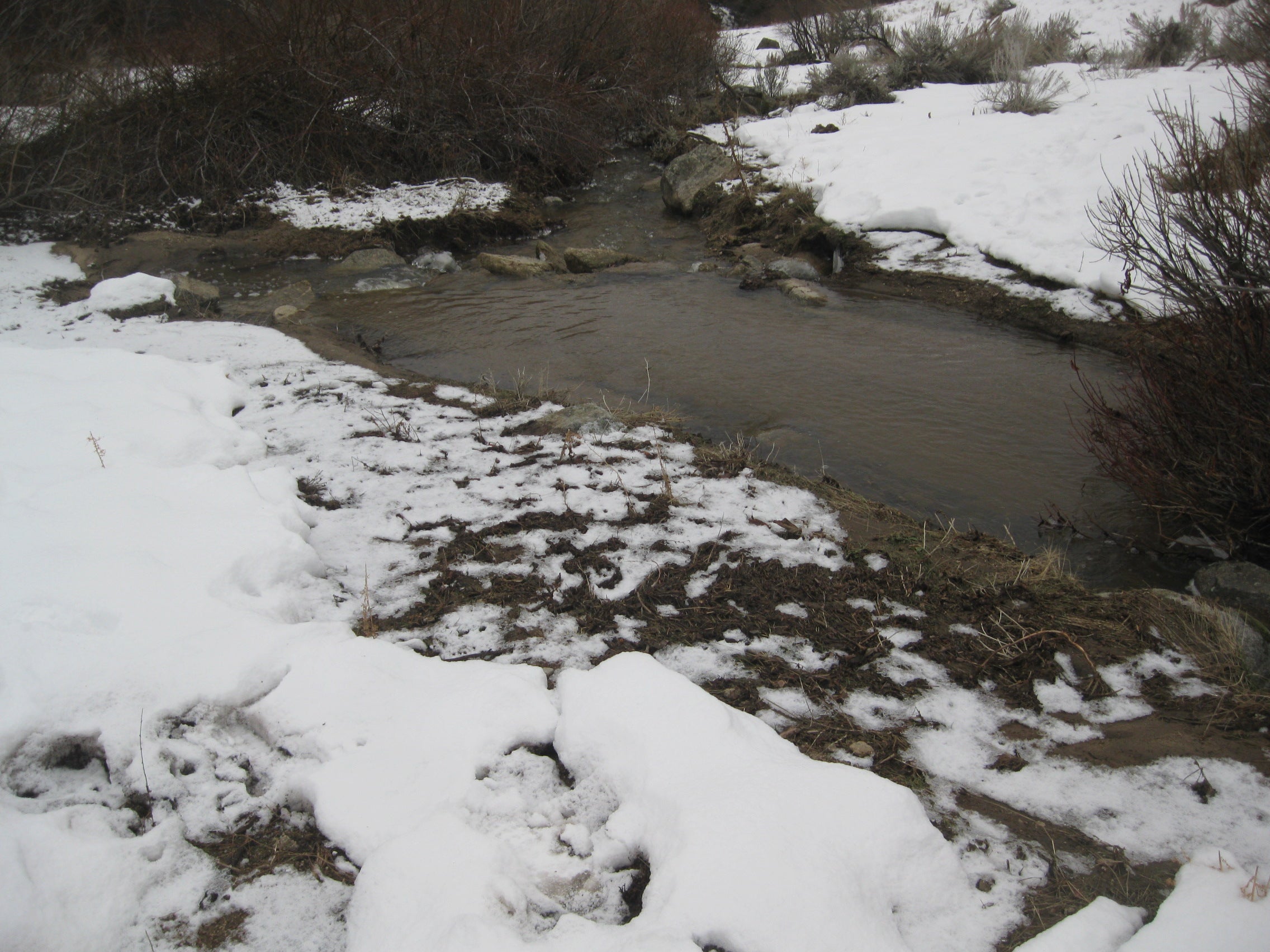
Estimate the flood flow at DCEW Lower Gauge using Manning’s equation for a storm that occurred in Jan 2011.

Project Files

• Calculations EXCEL workbook

Requirements and Connections

• Products of this exercise may be used by the Watershed Water Balance exercise.
• This exercise references stream instantaneous measurements of stage (and discharge) and DCEW Lower Gauge rating curve.
  

Manning’s Equation

Manning’s equation calculates the average velocity, U, of uniform flow in an open channel based on channel properties:

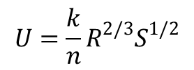
where R is the hydraulic radius (L), S is the channel slope (L/L), n is Manning’s roughness coefficient, and k is a unit conversion factor (k = 1 if R is in meters and U is m/s; k = 1.49 if R is in feet and U in ft/s).

The channel discharge can be computing by multiplying U by the channel cross section area (A),

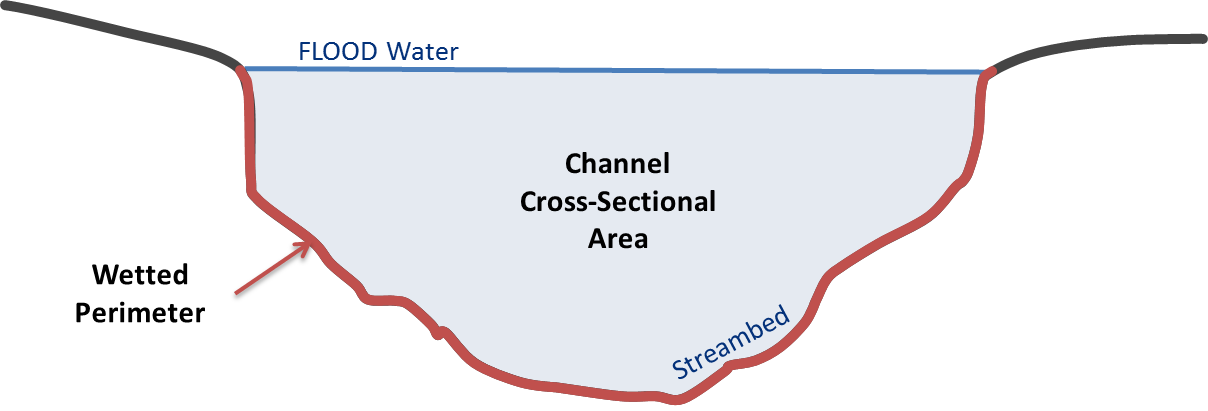
The hydraulic radius is computed as the cross-section area, divided by the wetted perimeter, P as indicated in equation 3:

The wetter perimeter is the distance along the channel bottom between water levels at each bank. Manning’s roughness, n, is a factor that characterizes the channel resistance. An internet search will reveal many different ways to estimate n. Ultimately, n is a site-specific factor that is determined by the scientist/engineer.

The Flood

On January 15, 2011 approximately 2 inches of rain fell on the Dry Creek Experimental Watershed, much of which was covered by snow. The combined rain and snowmelt produced a depth of streamflow approximately 2 ft higher than the highest stage for which we had a discharge measurement, rendering the stage-discharge relationship for the Lower Gauge unreliable (see Streamflow Measurement Exercise for an explanation of stage-discharge relationships). This flood presented an opportunity to add a very high water point to the rating curve. We know the stage from our instream datalogger, but  nobody was in the stream making measurements during the flood. Instead of using the velocity-area gauging method, we used Manning’s equation in a forensic sense to estimate discharge. To do so, field crews walked a section of the stream near the Lower Gauge and identified high water marks. Indicators of high water included debris clinging to brush, erosion scours, and anything else that gave clues to the highest height that water reached. The field crews then selected two locations along the channel reach and measured the shape of the flooded cross-sections. Each cross-section survey was completed by setting a survey instrument in line with the cross-section, and then measuring the elevation of the ground surface or stream bed at increasing distances away from the station, perpendicular to the channel. The distance and elevation drop between cross-sections along the stream were also surveyed to calculate channel slope.

Goal

Estimate the peak flood flow at DCEW Lower Gauge from the January 15, 2011 storm event.

Instructions

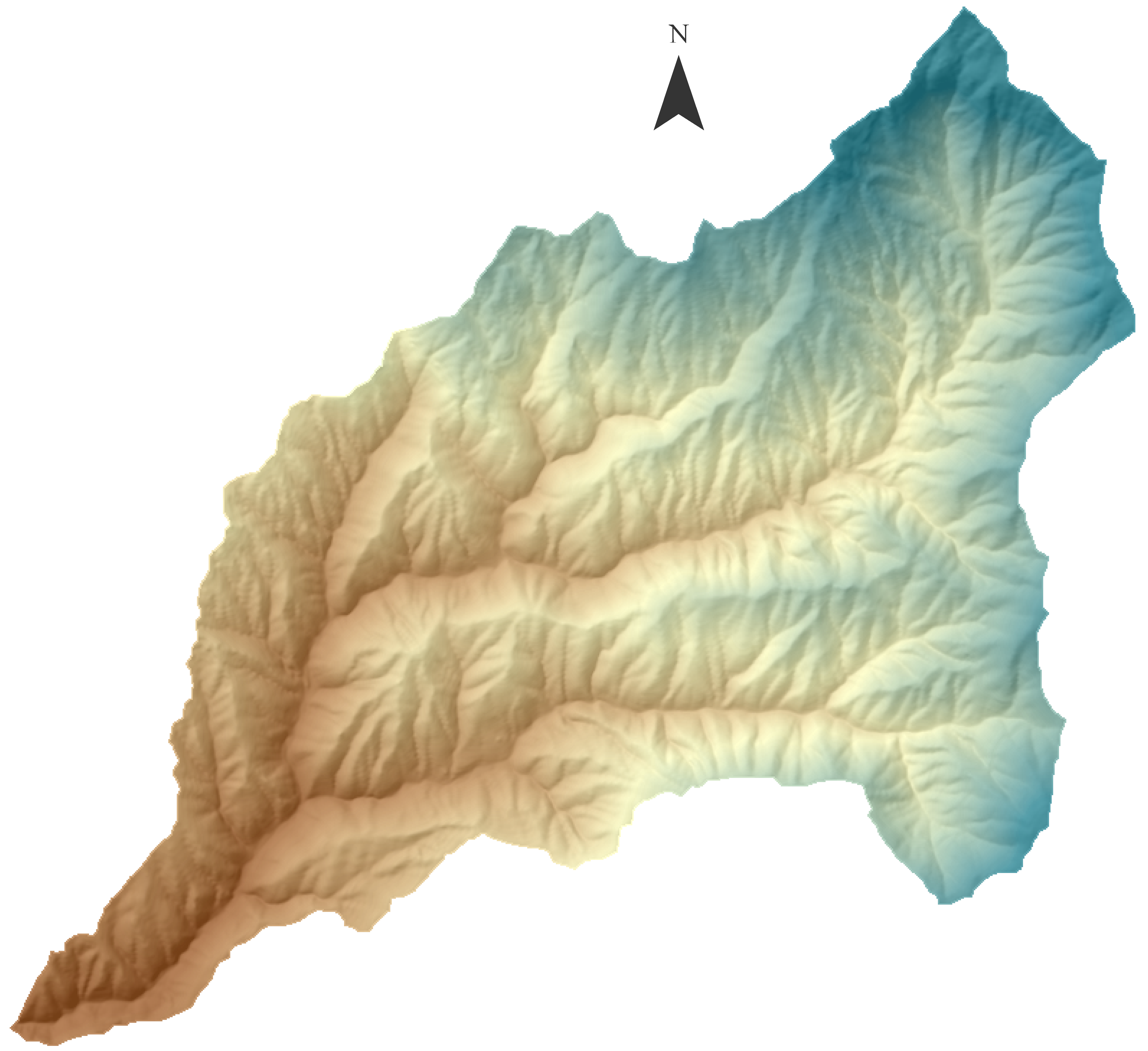
The instructions below outline specific steps to complete the exercise based on the fieldwork which was conducted near Lower Gauge. The field crew identified the flood water marks on each bank and then, two locations were used to survey the shape of the flooded channel resulting in an UPstream cross-section and DOWNstream cross-section. In the workbook provided, these cross-sections are automatically plotted in the “FloodFlow Calculation” tab.

Project Files

• Calculations EXCEL workbook

1. Cross-section Station Calculations

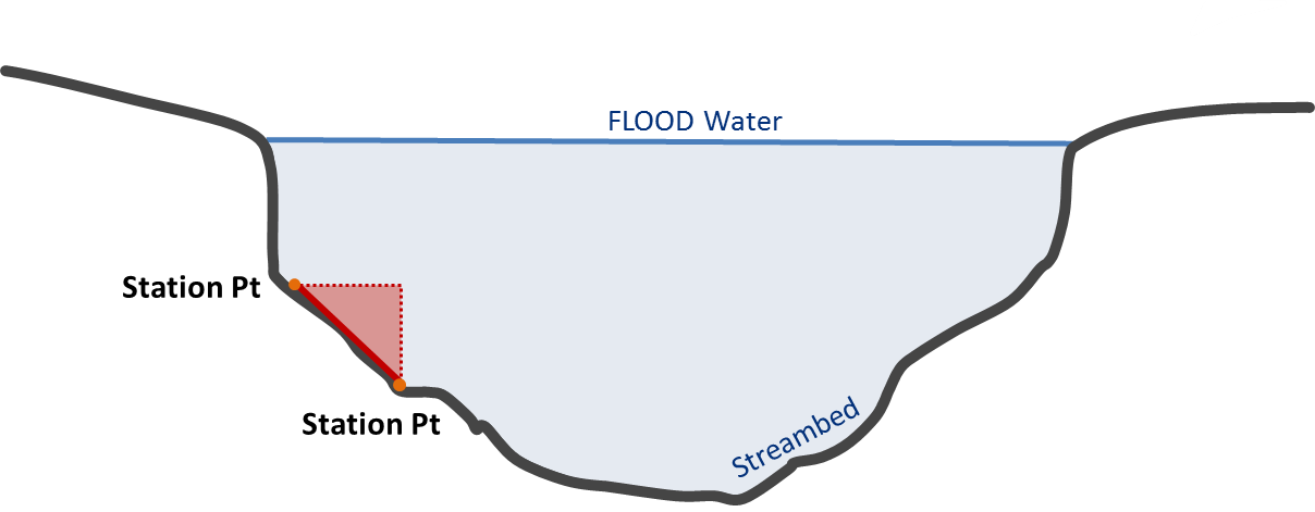
1. High water marks (a.k.a FLOODline) are identified in the ‘Field Notes’ column. Calculate the average elevation of the high water marks on the right and left banks. Enter the calculated value in the ‘Average FLOODline Elevation (m)’ of the red table of the appropriate UPstream/DOWNstream cross-section.
2. Calculate the ‘Flood Water Depth (m)  for each station in column G
3. Calculate the ‘Wetted Perimeter (m) of the channel by using Pythagorean theorem at each channel section as illustrated in figure on the right.
4. Calculate the ‘Cross-sectional Area (m²)’ of the flood flow by multiplying the width of each section and the average flood water depth of each section.

2. Channel Slope Calculations

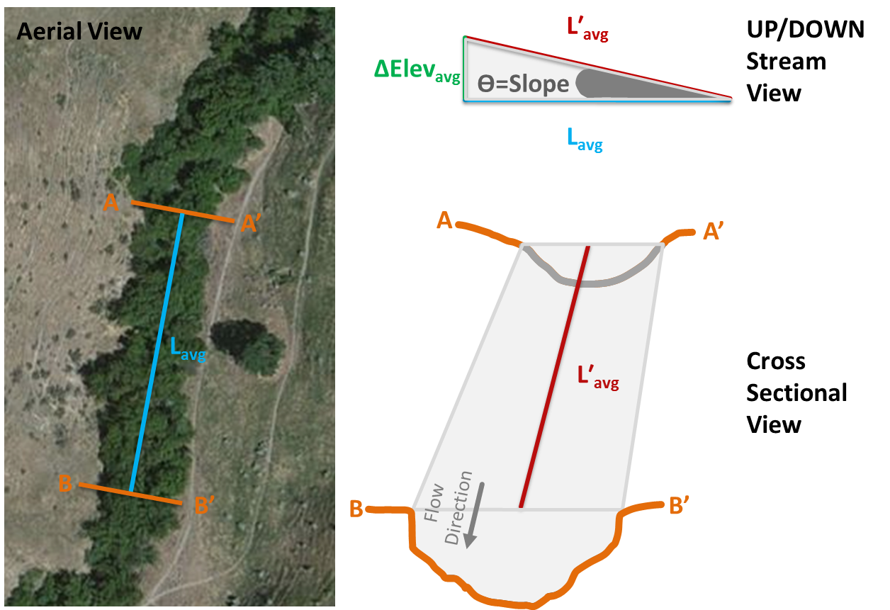
In the orange table, calculate

1. ‘ΔElevation_avg‘ between the UPstream and DOWNstream water surface elevations
2. ‘Channel Slope (m/m)’

3. Manning’s Calculations

For each of the cross-sections in its corresponding red table, complete the following

1. Estimate ‘n:Manning’s Roughness Coefficient’ .
   There are many ways to do this. Here, you will use this published table provides ranges of n for different stream descriptions. At the survey location, Dry Creek can be considered a mountain stream with steep banks. There is some vegetation in the channel in places,  brush and trees on the banks are submerged at high stages. The stream bed is composed of cobbles and boulders. Enter your value in the red table.
2. Calculate the total wetted perimeter in the appropriate cell by summing the wetted perimeter of all sections (determined in 1c).
3. Calculate the total cross-sectional area in the appropriate cell by summing the areas of all sections (determined in 1d).
4. Enter S: Channel Slope (m/m)’ which was determined in 2b.
5. Compute the hydraulic radius of the flooded channel in the appropriate cell.
6. Enter K: Because our survey data are in meters, K = 1.
7. Compute Q in m3/s using Manning’s Equation. Convert your Q value to cfs.

4. Compute Q Using a Rating Curve

At a permanent gauging station, a stage-discharge relationship (also called a Rating Curve) is used to convert continuous records of stage into continuous records of Q (See Streamflow Measurement exercise for background). To construct a rating curve, instantaneous streamflow measurements are made at various stages. A power function is then fit to the range of stage-discharge pairs. The power function is then used to predict Q for all stages. However, the equation should not be used to calculate Q for stages higher than the highest stage for which there is a measured Q.

The “Rating Curve” workbook tab contains several measured stage-discharge pairs. Note that the highest stage for which we have a corresponding measured discharge was 2.12 ft (which equates to 37.6 cfs). Peak stage for this exercise’s flood at the LG station was 4.18 ft. To illustrate the problem, you will use the rating curve to compute Q for the high stage.

1. On the automated scatter plot, add a Power Function trendline to the plot. Select the option to display the equation on the plot.
2. Use the equation to compute Q.

5. Discussion Questions

Compare your discharge estimate derived from Manning’s equation to that derived from the rating curve. Discuss reasons for differences.

6. Deliverables

1. Each cross-section’s Manning Equation results (red tables in the “FloodFlow Calculation” tab)
2. The rating curve Q calculations (red table in the “Rating Curve tab”)
3. Answers to discussion questions as assigned by instructor